Gradient descent:
It is an optimization function to find the minimum of a function. It is used for error optimization, so as the error value decreases, the output leads to convergence.
This decreasing error value is us, trying to find the minima or the smallest possible value. Once we find the minima, that’s our point of convergence, that’s where our code ends.
Gradient is essentially just a partial derivative, the tangent to a curve, it points to the direction of minima.
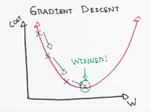
A simple gradient of weight and cost function(explained below). Here we can see the curve falling slowly, step by step(learning rate), and when it touches minima Phew! Phew! Phew!, it won.
Convergence:
In ML, convergence refers to having approximately equal values for desired output, and actual output.
Why gradient descent?
If a data set is too homogeneous, after training the model becomes “too fit” to the data, that’s overfit.
Its tough to generalize!, If an arbitrary data point came out of the context, the model cant predict accurately! the training data is not diverse!
generalization is giving near accurate prediction for any random value.
gradient descent help to solve this, instead of giving an immediate solution, it iteratively sets output, so that it can achieve desired output in future! error correction! feedback!
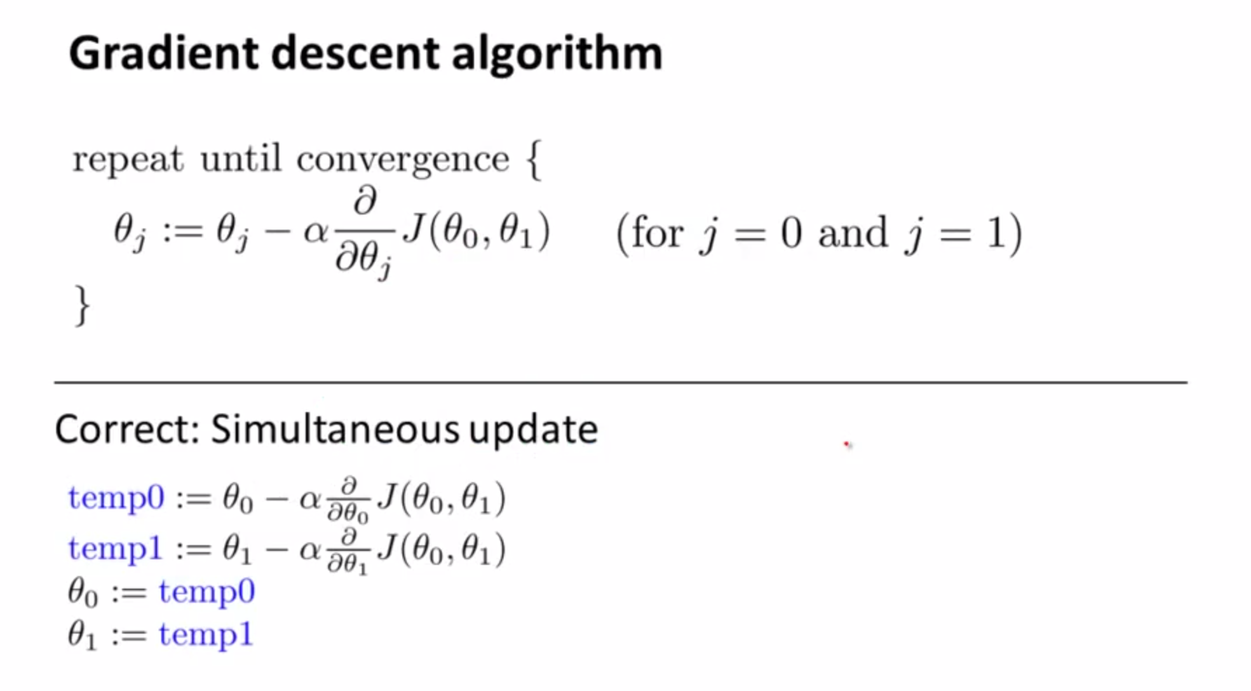
The variable referred here as weight, is actually the main parameter whose value is adjusted. In value update, we can see an alpha(α) which is the learning rate. And then there is a gradient of two inputs, θo and θ1.
Learning rate:
It is a hyperparameter which determines how fast a model trains. If its value is too low, too slow to converge and too high, the model will never converge. So, find optimal! and the only way is to guess and check.
Now the most important part!
Implementing gradient descent in Linear Regression:
Let’s see for a multidimensional Linear system. Now a single dimensional linear equation appears like this:
y=mx+c
Whereas a multi-dimensional is like this:
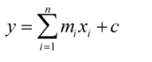
Here, we are evaluating the value of y, by taking summation of all the values of “mx”. Here m = weight, x= input, c= constant/bias.
From this form, we compute our cost function or the average mean square error value, by comparing the actual value of y, with the predicted value.
the cost function is given by:

Now, we are doing gradients!
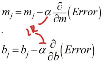
Partial derivative of the error function, error(m,b) with respect to weight(m) and bias(b), gives:

Now, the last step.
Apply gradient descent to update values of weight and bias!
Refer to Gradient Descent Algorithm.
So iteratively, the weight and bias gets updated, and as a result the error keeps on decreasing, eventually moving to convergence!
Disadvantage:
Though gradient descent is the sweet spot for Backpropagation, still its less preferred because of its minima issue.
It hovers around a particular local minima, ignoring other minima(s), there may be some other minima, where the value can reach far below this one. Those are the global minima, the situation arises when we consider 100s of features, a big cluster of unlabelled data.
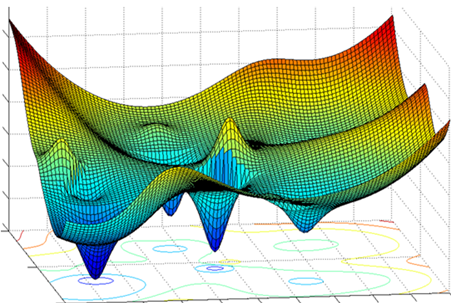
We can see there are numbers of local minima, and one of them is global minima.
We need to frame our model in such a way that it lands on the distribution featuring global minima!
MYTH:
Algorithms are easy to understand, but hard to implement! NO, the situation is just the opposite.
That’s all folks! If you love this, give thumbs up and some feedback too.
